August 31, 2026
Random In vs. Random Out: Evaluating Initial State Variance against Token-Wise Sampling in Open-Weight LLMs
A few weeks ago, Dan Wood wrote a LinkedIn post that I found interesting. He was thinking about Latent Space Reasoning and framed it in a way I hadn't seen before: Random In vs Random Out.
The idea is simple. When you want an LLM to explore different solutions to a problem, you have two basic choices for where to inject randomness:
- Random Out is what everyone knows. And it's temperature sampling. The model picks the next token with some randomness at every step. Set temperature to 0.7, and you get slightly different outputs each time.
- Random In is different. Instead of randomness during generation, you inject Gaussian noise into the input embeddings before the model starts generating. Then you run inference at temperature=0. It's fully deterministic. The randomness is front-loaded.
Dan's observation was that these two are structurally the same idea, just applied at different moments. And that Latent Space Perturbation is basically Temperature Annealing compressed into a single pre-token injection.
I read that and wanted to test it.
Why Random Out Has a Problem
Think about it like writing a proof. You write one line, check it, then write the next. If line 3 is wrong, everything after it is downstream of that mistake.
Temperature sampling is like writing the entire proof without stopping to check. If one step goes slightly wrong, the next step builds on that wrong step, and the one after builds on that, and so on. The errors compound. This is not hypothetical. It is why increasing temperature too much produces outputs that start coherent and then slowly drift into nonsense.
Random In sidesteps this. You perturb the starting state once. Then the model reasons from that perturbed starting point cleanly, at temperature=0. In this approach, each perturbation gives you a different "angle" on the problem, but the execution from each angle is deterministic.
The Experiment
I tested this on Qwen/Qwen2.5-7B-Instruct, running on Kaggle's free T4 × 2 GPUs. I tested with five problems across different categories (logic, code, math, system design, and strategy). For each problem, I ran the model at five different noise scales: 0.0, 0.02, 0.05, 0.1, and 0.2.
noise_scale = 0.0 is the clean baseline. The model produces identical output every single time.
To measure what happened across trials, I used three metrics:
- Self-BLEU - how similar the three outputs are at the word level. Lower means more lexically diverse.
- Semantic Distance - how far apart the outputs are in meaning. Higher means more conceptually distinct.
- Coherence Collapse Rate - fraction of outputs that are empty, too short, or clearly off-topic. Higher means the model broke.
Experiment Outputs
| Problem | Noise_Scale | Self_BLEU | Semantic_Distance | Collapse_Rate |
|---|---|---|---|---|
| Logic | 0.00 | 1.0000 | 0.0000 | 0.0000 |
| Logic | 0.02 | 0.5511 | 0.1098 | 0.0000 |
| Logic | 0.05 | 0.0000 | 0.0000 | 0.6667 |
| Logic | 0.10 | 0.0000 | 0.0000 | 1.0000 |
| Logic | 0.20 | 0.0000 | 0.9586 | 0.3333 |
| Math | 0.00 | 1.0000 | -0.0000 | 0.0000 |
| Math | 0.02 | 0.6724 | 0.0699 | 0.0000 |
| Math | 0.05 | 0.0000 | 0.8632 | 0.6667 |
| Architecture | 0.00 | 1.0000 | 0.0000 | 0.0000 |
| Architecture | 0.02 | 0.3082 | 0.0698 | 0.0000 |
| Architecture | 0.05 | 0.0000 | 0.0000 | 1.0000 |
| Strategy | 0.02 | 0.4937 | 0.0869 | 0.0000 |
| Code | 0.02 | 0.9869 | 0.0003 | 0.0000 |
At noise = 0.0, all three trials are word-for-word identical. Self-BLEU = 1.0. The model is a fixed function. It gave same input, same output, always.
At noise = 0.02, something changes. Self-BLEU drops. And semantic distance rises. The three outputs are now genuinely different from each other, sometimes different approaches. But Collapse Rate stays at 0.0 across every single category. The model is still coherent. It still remembers the question.
At noise = 0.05 and above, things break fast. Most categories hit Collapse Rate = 1.0 by noise = 0.1. At noise = 0.2, the Logic trials produced outputs in Chinese. The Math trials answered an entirely different problem. The model had forgotten what it was asked.
The figures show this clearly:
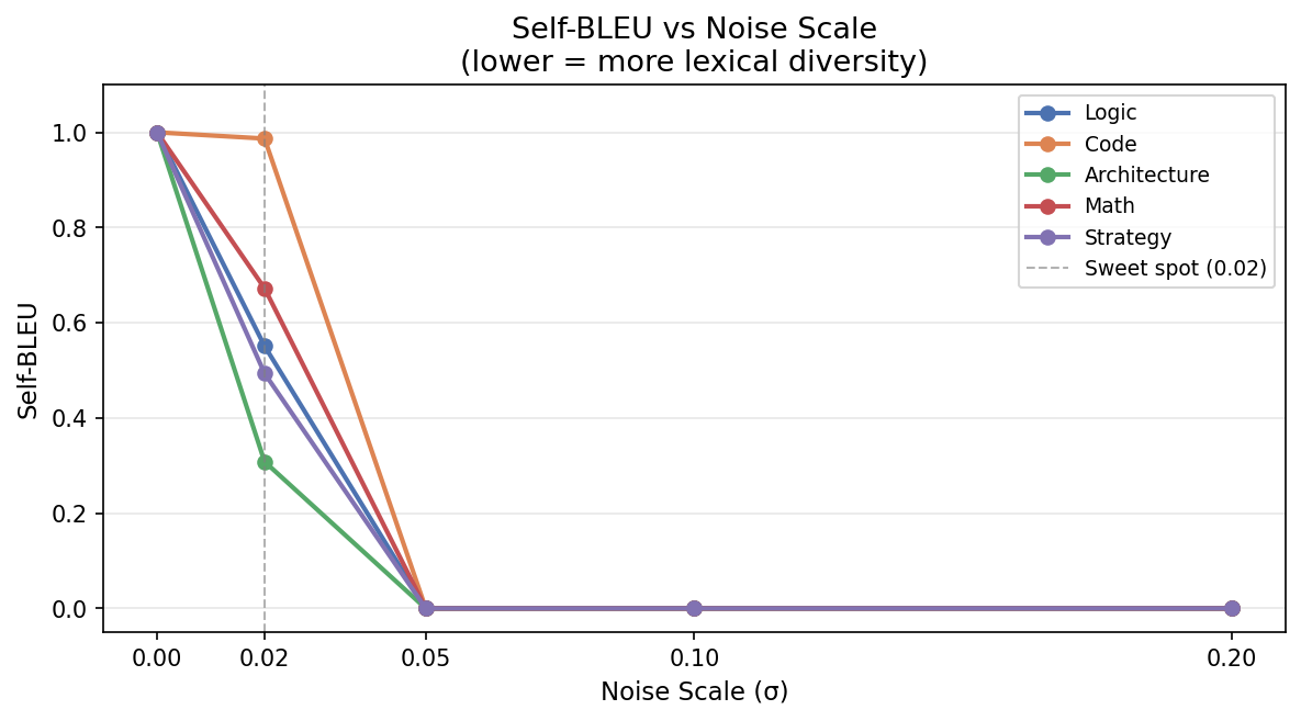
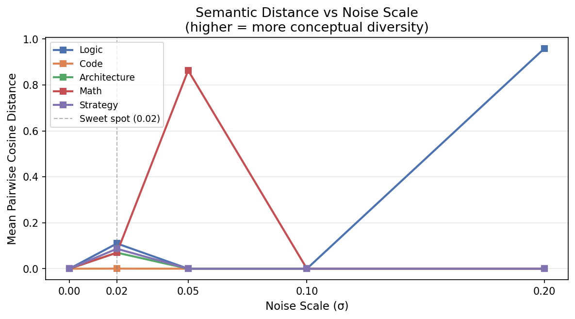
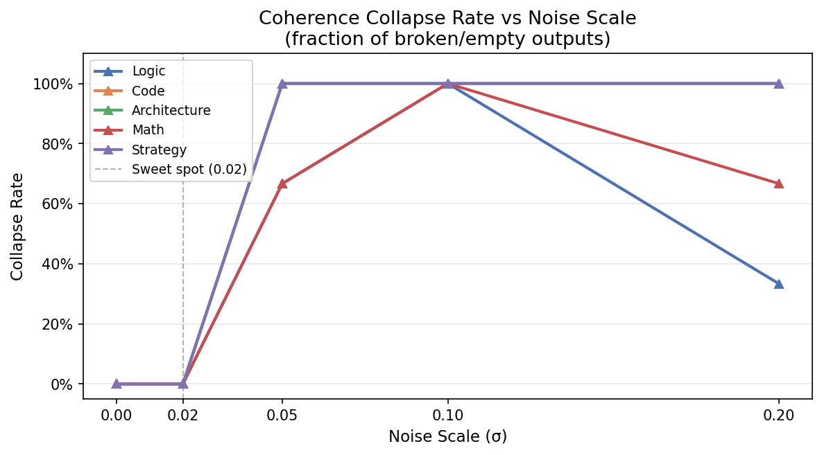
There is a very narrow window, around noise = 0.02, where latent perturbation gives you genuine diversity without breaking anything.
Too little noise: identical outputs, no exploration at all.
Too much noise: the model forgets the question entirely.
Just right (0.02): real diversity, zero collapse.
What is interesting is how sharp this boundary is. The jump from noise = 0.02 (Collapse Rate = 0.0) to noise = 0.05 (Collapse Rate = 0.67 to 1.0 depending on category) is large. There is not a gradual degradation.
This makes sense if you think about how token embeddings work. The model has learned a very specific region of embedding space where inputs are "valid", where the geometry of the embeddings maps to coherent language. A tiny perturbation moves you to a different point within that region. A large perturbation throws you outside it entirely, and the model has no idea what to do.
What This Connects Back To
Dan's broader post was about something more ambitious, the idea that a model could learn to control its own temperature schedule. Instead of an external system managing when to be random and when to be precise, the model itself could emit a <temp=0> token the moment it locks down a strategy. Or <temp=x> at moments where divergent thinking is useful.
That is interesting and I think correct in direction. What this experiment adds is that the where matters as much as the when. Injecting randomness before inference is fundamentally cleaner than injecting it during inference, because you avoid compounding errors entirely.
The tradeoff is sensitivity. Random Out (temperature sampling) is forgiving, you can set temperature to 0.7 and get reasonable outputs across a wide range. Random In has a much narrower operating window. Noise = 0.02 works. Noise = 0.05 does not. That sensitivity is a practical problem if you want to use this in production.
Limits of This Experiment
A few things I want to be honest about.
This is one model, one size, five problems, three trials each. Whatever I found, noise ≈ 0.02, is specific to Qwen2.5-7B-Instruct. A different model, a different size, or a different embedding dimension might have a completely different sweet spot. Or no sweet spot at all.
I also did not measure quality, only diversity and coherence. The outputs at noise = 0.02 are more diverse than noise = 0.0, but I did not check whether they are better. A more rigorous experiment would score each output against a ground truth and ask: does diversity here actually translate to finding better solutions?
That is the real question Dan's work is pointing at. He is running 100 problems × 20 perturbations on GSM8K, which is a benchmark with known correct answers. That is where you can actually measure whether the diversity is useful diversity.
Code and Results
Everything is on GitHub, the experiment code, analysis script, raw results CSV, and generated figures.
github.com/byGanesh/latent-noise-reasoning
The experiment runs on Kaggle free tier (T4 × 2). The analysis runs on CPU. If you want to reproduce it or try a different model, the code is straightforward to modify.
Thanks to Dan Wood for the framing that started this.